
From Raw to Refined
The First 30% of Your Data Science Journey - Feature Engineering

Feature engineering is the backbone of any data science project. It transforms raw data into a useful format that machine learning models can digest. Think of it as prepping ingredients before cooking—a vital step to ensure your dish turns out delicious. This guide is my way of making feature engineering approachable and easy to understand.
[ P.S. Happy Independence Day, Pakistanis :) ]
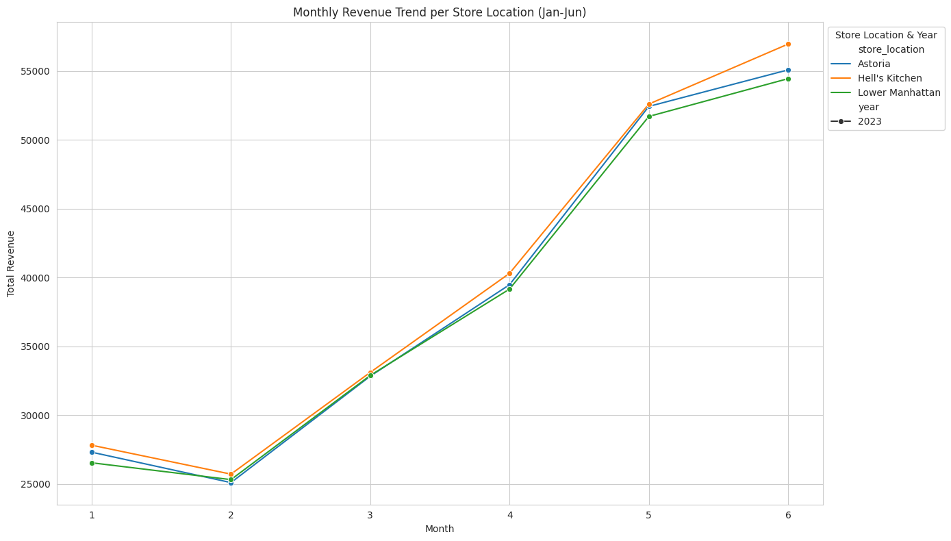
[For a practical example, check out my GitHub project on coffee shop sales data. It showcases some of these techniques in action, answering key business questions through EDA.]
Step 1: Exploratory Data Analysis (EDA)
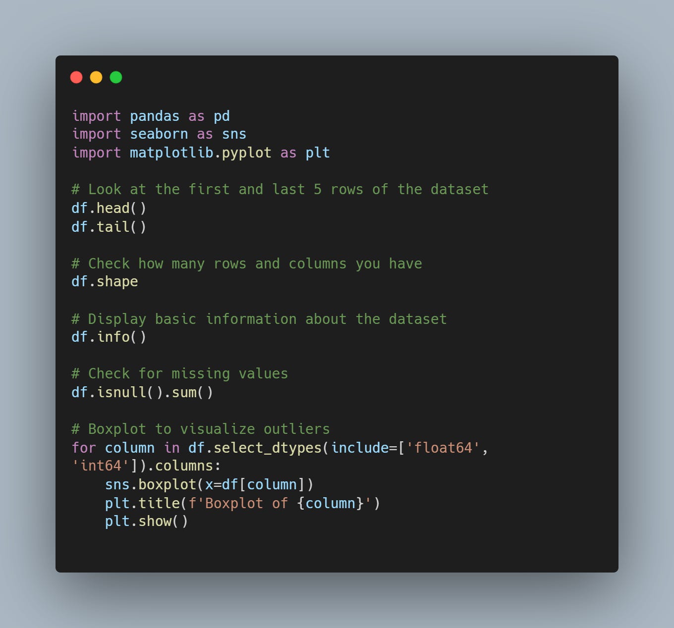
Before transforming data, you need to understand it. EDA is your chance of acting like Sherlock Holmes but data science version—uncovering the hidden secrets of your dataset. I generally look at:
Shape of the Data: Check how many rows and columns you have. This gives you a sense of the dataset's size and complexity.
Numerical Features: Use histograms and PDFs (probability density functions) with Seaborn to visualize distributions. This helps in understanding the spread and central tendencies of your data.
Categorical Features: Count unique values and visualize with bar charts. This helps in understanding the distribution of categories and identifying any dominant or underrepresented classes.
Missing Values: Use heatmaps to spot missing values. Identifying missing data early can save a lot of headaches later.
Outliers: Identify outliers with boxplots. Decide whether to clean or keep them. Outliers can significantly affect the performance of your models.
Step 2: Handling Missing Values
Missing values are common, but they’re not the end of the world. You can wish they didn’t exist or you could handle them - your choice.
Here are five techniques I’ve used the most:
Mean Imputation: Replace missing values with the mean of the column. Simple but can distort data if outliers are present.
Median Imputation: Similar to mean but more robust against outliers.
Mode Imputation: Good for categorical features.
Forward/Backward Fill: Propagate next or previous values, useful for time series data.
Dropping: Sometimes, it’s best to drop rows or columns with too many missing values. I usually drop columns I don’t need.
Step 3: Handling Imbalanced Datasets
An imbalanced dataset can mislead your model. Here’s how to fix it:
Resampling: Over-sample the minority class or under-sample the majority class.
SMOTE (Synthetic Minority Over-sampling Technique): Generate synthetic samples for the minority class.
Class Weight Adjustment: Modify the weights in your model to balance classes.
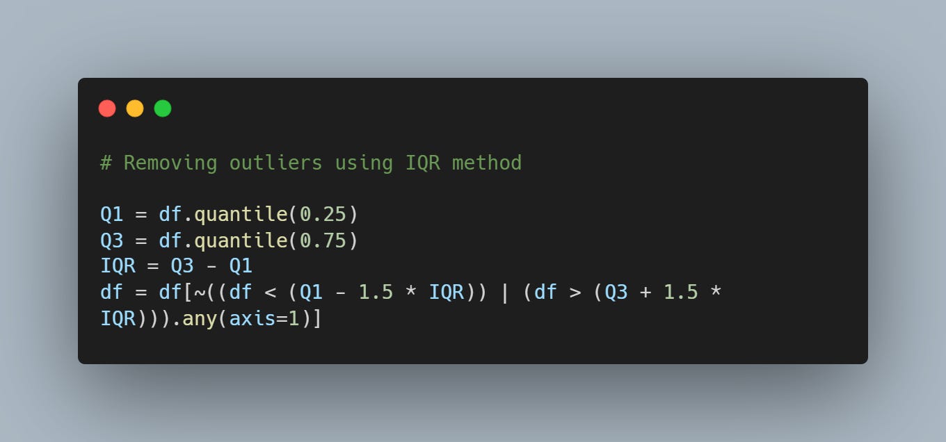
Step 4: Treating Outliers
Outliers can skew your results. There are a lot of techniques out there but I’ve used these the most:
Z-Score: Standardize data and remove values beyond a certain threshold.
IQR (Interquartile Range): Remove values outside 1.5*IQR from the first and third quartiles.
Step 5: Scaling Data
Scaling ensures all features contribute equally. Common methods are:
Standardization: Transform data to have zero mean and unit variance.
Normalization: Scale data to a range of [0, 1].
Step 6: Converting Categorical Features to Numerical
Machine learning models love numbers. Convert categorical features using:
Label Encoding: Assign a unique integer to each category.
One-Hot Encoding: Create binary columns for each category.
Post Feature Engineering:
Feature Selection: Use correlation matrices or feature importance scores to select relevant features.
Feature Creation: Combine existing features to create new ones that better capture patterns in your data.
Remember, in data science, the magic often lies in the prep work.
Thank you for reading. If you found this helpful, stay tuned for more insights and tips on navigating the world of data and cloud computing.